Earth’s surface is a complex, irregular expanse full of peaks, valleys, natural habitats, and human-made objects. With modern surveying techniques, computing power and sophisticated software it’s possible to visualise and inspect these features in ways that reveal their history, structure, interactions and potential beneficial exploitation. Uses include estimating areas most vulnerable to sea-level rise, spotting unauthorised developments, identifying land use (arable, pasture, forestry, moorland), and monitoring the type and condition of surface vegetation.
There are many ways to model elevation, but the three most useful are:
- DEM – Digital Elevation Model
- DSM – Digital Surface Model
- DTM – Digital Terrain Model
DEMs are digital representations of the earth’s topographic surface. They’re a “bare-earth” product because they do not include surface features like buildings and vegetation. In contrast, DSMs capture both the natural and built/artificial features of the environment. Examples include trees, crops, power lines and buildings.
DEMs and DSMs can be combined to good effect. For instance, forestry managers often exploit the difference between the DEM and DSM of an area to reveal tree canopy height, density and spread. More impressively, given data of sufficient accuracy they can measure the crown diameter/area, root spread and condition of individual trees. This facility allows forestry managers to limit the number, frequency and scope of on-site inspections, thus reducing manpower requirements and associated costs.
To make sense of DEM/DSMs it is often helpful to create digital models or 3D representations/visualisations of a terrain’s surface from the elevation data. These are DTMs which typically include vector features of the natural terrain, such as rivers and ridges. A DTM may be interpolated to generate a DEM, but not vice versa.
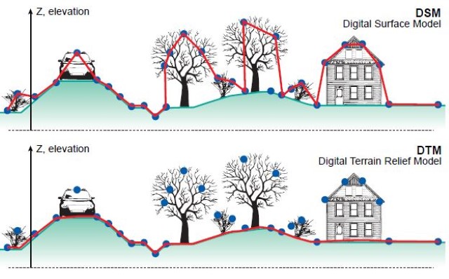
Table of Contents
Use of QGIS to create a Digital Terrain Model
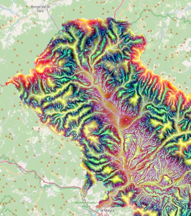
The best free software for creating DTMs from elevation data is QGIS, and the most accurate dataset for Tuscany is that available for download from the Regione Toscana GeoBlog website.
The process is as follows:
- Install QGIS.
- Install the QuickMapServices plugin in order to access OpenStreetMap and display an underlying basemap.
- Install the Relief Visualisation Toolbox plugin (needed to produce the terrain model).
- Install suitable terrain elevation data.
- Adjust the CRS (Coordinate Reference System) if necessary.
- Produce the Digital Terrain Model.
For reasons I have yet to establish, I have not been able to create a DTM using data downloaded via the the NASA SRTM plugin – all I get is an error message. However, I have had success with the LiDAR derived data available from the Regione Toscana GeoBlog website.
Installation of QuickMapServices plugin to access OpenStreetMap
- Launch QGIS.
- From the “Project” tab on the menu bar, select “New” to create a new project.
- From the “Project” tab on the menu bar, select “Save” to save the project.
- Select “Plugins” from the QGIS menu bar.
- Select “Manage and Install Plugins”.
- From the search bar of the Plugins window, type and search “QuickMapServices”.
- Select “Upgrade” to download a new version of the plugin, where applicable.
- Click “Install” to install the “QuickMapServices” plugin.
- From pool of tools on the menu bar, select “Web”.
- Toggle to “QuickMapServices” and select OSM to import the OpenStreetMap basemap.
Installation of Relief Visualization Toolbox (RVT) plugin to generate the Terrain Model
- Select Plugins from the menu bar.
- Select Manage and install plugins.
- From the search bar of the Plugins window, type and search for “Relief Visualization Toolbox”.
- Select “Upgrade” to download a new version of the plugin, where applicable.
- Click “Install” to install the RVT plugin.
Download the Digital Elevation Data & use the RVT to Compute
- Access the Regione Toscana GeoBlog website.
- Download the dataset of interest (eg DTM 10×10 m – Provincia di Massa-Carrara). This will be contained in a ZIP file. Double click to open and then copy out the two files within. One file will be a PDF containing licence information together with coordinate reference system details (typically Gauss-Boaga Fuso Ovest (EPSG:3003)). The second file will have an ASC extension and will contain the required elevation data.
- In QGIS go to “Layer”, then “Add Layer”, then “Add Raster Layer”. Under the “Raster dataset(s)” tab navigate to the ASC file referred to above. Then click the “Add” button in the bottom right hand corner. The data should now appear in the “Layer” panel on the left hand side of your screen, suitably labelled.
- Since the default CRS for QGIS is WGS84 and not Gauss-Boaga you are now going to have to convert the data. To do this, click on “Raster”, then “Projections”, then “Warp (Reproject)”. A box pops up. The “Source CRS” should be set to “EPSG: 3003 – Monte Mario/Italy zone 1”, and the “Target CRS” should be set to “EPSG: 3857 – WGS84 Pseudo- Mercator” (to match OpenStreetMap). Under “Advanced parameters” give the reprojected data file a name (eg MS_Reprojected_WGS84) and a location. Ignore the other parameters and click on “Run”. Conversion to the new CRS will take some time!
- After the CRS conversion process has finished, click on the “Raster” tab, then the “Relief Visualization Toolbox” option, and select “Relief Visualisation Toolbox”. In the window that pops up, select the reprojected data layer, then “Select all”, then “Start”. Be warned that the calculations can take some considerable time.
- The visualizations appear as TIF files in the “Layer” window.